Beam-Beam Elements and Dipolar Effects in MAD-X (In Construction...)

In this section, we describe the way dipolar effects are handled by the different MAD-X modules depending on their source, one of the highlight being the beam-beam (BB) element. To see the details of the code, please refer directly to the notebook itself, that can be found here.

I - Preliminaries

1) MAD-X through cpymad in a jupyter notebook

From your favourite ipython notebook environment - let's call it SWAN - you can simply import the cpymad package by running:

from cpymad.madx import Madx

Then you need to launch a MAD-X instance by:

madx = Madx()

2) Beam-beam Kick: Analytical Reference

In order to compare the results of MAD-X with the theory, we use this formula [1]: $$ \Delta x' (x,y) = \frac{2 r_p N_p}{\gamma_r}\frac{x}{r^2}(1 - e^{-r^2/2\sigma^2}), $$ where $r_p$ is the classical proton radius ( $r_p \simeq 1.53\cdot10^{-18}$ ~m), $N_p$ is the bunch intensity and $r$ is define as $r = \sqrt{x^2 + y^2}$ and $x$ , $y$ represent respectively the horizontal and vertical positions of the strong beam in the weak beam reference frame. Note that indeed there is a sign difference between the proposed formula and the one one can find in the reference. An adaptation to fit the MAD-X conventions was necessary.

In order to simplify the problem, we consider a perfect horizontal crossing (e.g, in IR5). The equation above therefore becomes $(y=0)$ :

$\Delta x' (x) = \frac{2 r_p N_p}{\gamma_r x}(1 - e^{-x^2/2\sigma^2}).$

3) About MAD-X: line/period, closed orbit/trajectory/reference orbit...

MAD-X is using a specific vocabulary to describe different situations or tools. Even though this document tries to deal with those concepts as clear as possible, the need of another specific page was needed. Find out more here.

II - Horizontal Kicker

In this first section, we will describe how an horizontal kicker acts a beam in MAD-X, comparing two situations: a line and a circular machine (period).

1) Transfer Line

In this first part, we build a simple transfer line composed of a simple drift in which we will install a horizontal kicker. In this case, it is clear that the $\beta$ -function is a parabola depending on the $\beta$ -function at the interaction point $\beta^*$ and on the longitudinal position $s$ :

$\beta (s) = \beta^* + \frac{s^2}{\beta^*}.$

We assume a $\beta^*$ of 25 cm, a beam energy of 6.5 TeV and a normalized emittance of 3.5 $\mu$ m. At this point we also assume that the strong beam is centered with respect to the weak beam reference. All together in Python:

betax_IP=0.25 # beta_x at the IP. The IP is the start of the sequence
betay_IP=0.25 # beta_y at the IP. The IP is the start of the sequence
positionBB=10 # position of the BB and end of the transfer lin
totalEnergy=6500 # beam total energy
emittanceNormalized=3.5e-6 # we assume same h/v normalized emittance
npart=1.15e11 # number of particle in the strong beam
xma=0 # x position of the strong beam center wrt the weak beam reference
yma=0 # y position of the strong beam center wrt the weak beam reference

gamma=particle.setTotalEnergy_GeV(6500)['relativisticGamma'] # from cl2pd import particle
betagamma=particle.setTotalEnergy_GeV(6500)['relativisticBetaGamma']
betax_BB=betax_IP+positionBB**2/betax_IP # we are in a drift
betay_BB=betax_IP+positionBB**2/betay_IP # we are in a drift
sigma_x=np.sqrt(betax_BB*emittanceNormalized/betagamma) 
sigma_y=np.sqrt(betay_BB*emittanceNormalized/betagamma)

One is now ready to build a simple transfer line in MAD-X. We define and install an horizontal kick HKICKER at 10 m from the interaction point. Our sequence is therefore simply composed of a drift in which a HKICKER is installed.

madx.input(
f'''
option,echo=false,warn=false,info=false;
myHKICK : hkicker, kick=1E-6;

lhc: sequence, l={positionBB};
myHKICK1 : myHKICK, at={positionBB};
endsequence;

beam, particle=proton, energy={totalEnergy}, npart={npart};
use, sequence=lhc;

option, bborbit=true;
twiss,betx={betax_IP},bety={betay_IP};
''');

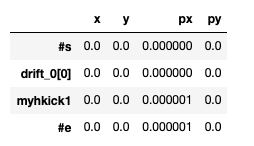
The obtained TWISS table contains the kick we implemented:

png

We now want to track particles through this line. This is done using the TRACK module of MAD-X. One has to determine a set of intial positions for the particles to track and an observation point (in this case, the HKICKER). In our example, the number or turns is set to 1. Using the cpymad module, we get:

points=51
x_range= np.linspace(-.002,.002,points)
myString=f'track, onepass={onepass};\n'
for myX in x_range:
    myString+=f'''start,x={myX};\n'''
myString+='observe, place=myBB1;run, turns=1; endtrack;\n'

One notices an interesting argument of the TRACK module: the onepass argument. This arguments either asks MAD-X to compute a closed orbit and to give the particle coordinates with respect to it (onepass set to False) or asks MAD-X not to compute any closed orbit and to give the particle coordinates with respect to the reference orbit (onepass set to True).

The results of the TRACK module are shown below, for both the cases about the onepass argument.

png

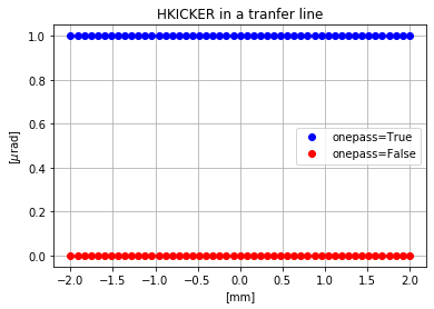
In the case where onepass is set to False, no kick is visible. The dipolar kick induced by the HKICKER is absorbed in the closed orbit and therefore the results of the tracking do not show any kick. In the opposite case, the kick is visible since the particle coordinates are given with respect to the reference orbit.

On the other hand, setting the onepass argument to False in the case of a transfer line does not make a lot of sense since by definition the lattice is not periodic and the concepts of turn are closed orbit do not apply. As stated by the MAD-X manual, this argument shall always be set to True for transfer lines. As we will see later, setting the argument to False in the case of a line does ask MAD-X to compute somehow a trajectory, but the algorithm can be very unstable, leading to inconsistent results, for instance, in the case of a beam-beam element.

2) Circular Machine

One can study a similar sequence, but including it in a period in which the computation of a closed orbit would make more sense. To do so, we are using the same transfer line and we close the machine using the MATRIX element in MAD-X. If one denotes $\beta_{1}$ the $\beta$ -functions at the kicker location, $\beta_{2}$ the $\beta$ -functions at the IP and $\mu_{12}$ the phase advance between the two (from the side of the rotation, and chosen such as the tunes of the machine are 0.31/0.32), the matrix can be defined by:

$R = \begin{pmatrix} \sqrt{\frac{\beta_{x2}}{\beta_{x1}}} \cos{(2 \pi \mu_{x12})} + \alpha_{x1}\sin{(2 \pi \mu_{x12})} & \sqrt{\beta_{x1}\beta_{x2}} \sin{(2 \pi \mu_{x12})} & 0 & 0 \\ \frac{\alpha_{x1} - \alpha_{x2}}{\sqrt{\beta_{x1} \beta_{x2}}} \cos{(2 \pi \mu_{x12})} - \frac{1 + \alpha_{x1} \alpha_{x2}}{\sqrt{\beta_{x1} \beta_{x2}}} \sin{(2 \pi \mu_{x12})} & \sqrt{\frac{\beta_{x1}}{\beta_{x2}}} \cos{(2 \pi \mu_{x12})} - \alpha_{x2}\sin{(2 \pi \mu_{x12})} & 0 & 0 \\ 0 & 0 & \sqrt{\frac{\beta_{y2}}{\beta_{y1}}} \cos{(2 \pi \mu_{y12})} + \alpha_{y1}\sin{(2 \pi \mu_{y12})} & \sqrt{\beta_{y1}\beta_{y2}} \sin{(2 \pi \mu_{y12})} \\ 0 & 0 & \frac{\alpha_{y1} - \alpha_{y2}}{\sqrt{\beta_{y1} \beta_{y2}}} \cos{(2 \pi \mu_{y12})} - \frac{1 + \alpha_{y1} \alpha_{y2}}{\sqrt{\beta_{y1} \beta_{y2}}} \sin{(2 \pi \mu_{y12})} & \sqrt{\frac{\beta_{y1}}{\beta_{y2}}} \cos{(2 \pi \mu_{y12})} - \alpha_{y2}\sin{(2 \pi \mu_{y12})} \end{pmatrix}$

Once each coefficient of the matrix is defined, one can implement our new circular machine in MAD-X using the following:

madx.input(
f'''
myHKICK : hkicker, kick=1E-6;
myMatrix: MATRIX, L=0, RM11={RM11}, RM12={RM12}, RM21={RM21}, RM22={RM22},
    RM33={RM33}, RM34={RM34}, RM43={RM43}, RM44={RM44};

lhc: sequence, l={positionBB};
myHKICK1 : myHKICK, at={positionBB};
myMatrix1: myMatrix, at={positionBB};
endsequence;

beam, particle=proton, energy={totalEnergy}, npart={npart};
use, sequence=lhc;

option, bborbit=false;
twiss;
option,echo=false,warn=false,info=false;
''');

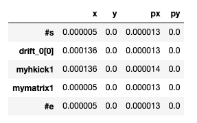
The TWISS table shows now a closed orbit that does not vanish:

png

And the results of the tracking are similar:

png

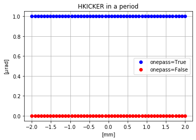
Both the options for the onepass argument are possible while using a period. But the rule remains the same. As output of the tracking module, the particles coordinates will be either given with respect to the computed closed orbit (onepass set to False) or to the reference orbit (onepass set to True).

The effect of the HKICKER dipole kick on a beam in MAD-X was pretty straight forward and was for us a simple introduction to the actual element we are trying to describe in this page. Indeed if the dipolar kick induced by a HKICKER is addressed is a straightforward way, this is not the case for the BB element.

III - Beam-beam element

1) General Remarks on the BB Element

We start by installing a BB element in a simple transfer line as defined in the previous section. The only changed compared to the previous example is that we replace the HKICKER by a BEAMBEAM element in the sequence.

madx.input(
f'''
option,echo=false,warn=false,info=false;
myBB : beambeam, charge=+1, sigx={sigma_x}, sigy={sigma_y}, xma={xma}, yma={yma}, bbshape=1, bbdir=-1;

lhc: sequence, l={positionBB};
myBB1: myBB, at={positionBB};
endsequence;

beam, particle=proton, energy={totalEnergy}, npart={npart};
use, sequence=lhc;

option, bborbit=false;
twiss,betx={betax_IP},bety={betay_IP};
''');

One of the line of interest in the code above is the setting of the bborbit flag to False. This means that the dipolar component of the BB kick is removed. We will come back to that point later, since at the moment the goal of this paragraph is to identify general properties of the BB element.

In the example above, the declared intensity correspond to the weak beam, not the strong. It therefore means that if this value is put down to zero, so will the kick.

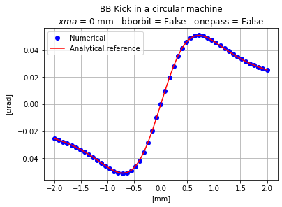
One can then track particles in this transfer line and see what is the kick they received as a function of their transverse position. Both numerical and analytical results are shown in the next Figure.

png

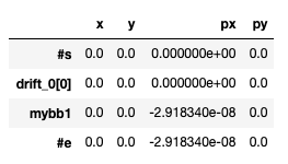
In this example, as mentionned before, the onepass argument is set to True since we are dealing with a line. The numerical results correspond to the analytical computation. Looking at the obtained TWISS table, one can observe that no kick is not present:

png

This is due to the fact that the bborbit flag is set to False and therefore the closed orbit (in the case of a line, the trajectory) vanishes.

Beam Intensity

As mentionned, the intensity defined by the user corresponds to the one of the weak beam that is the beam we are tracking. If one wants to increase the intensity of the strong beam in order for instance to increase the kick, the trick consists in modifying the charge of the beam-beam element. For instance in the next example, the charge of the beam-beam element is doubled:

madx.input(
f'''
option,echo=false,warn=false,info=false;
myBB : beambeam, charge=+2, sigx={sigma_x}, sigy={sigma_y}, xma={xma}, yma={yma}, bbshape=1, bbdir=-1;

lhc: sequence, l={positionBB};
myBB1: myBB, at={positionBB};
endsequence;

beam, particle=proton, energy={totalEnergy},npart={npart};
use, sequence=lhc;

option, bborbit=false;
twiss,betx={betax_IP},bety={betay_IP};
''');

And the kick is indeed doubled as expected:

png

In the same way, one can put the charge of the BB element to zero. This will have as a consequence to switch off this element, and therefore no kick is observed. Finally, one can change the charge sign of the BB element. The obtained kick through the traccking will be the same, with a change of sign.

Direction of the opposite beam

In the BB element, one argument (bbdir) sets the direction of the strong beam. By default, this argument is set to -1: beams move in opposite direction as in a collider. The Lorentz force enhances the BB interactions. If this argument is set to +1, the beams move in the same direction. This is for instance used in the case of an electron cooler. First, let us simply set the bbdir to +1, not defining any other beam, and leaving the charge of the BB element to +1.

madx.input(
f'''
myBB : beambeam, charge=+1, sigx={sigma_x}, sigy={sigma_y}, xma={xma}, yma={yma}, bbshape=1, bbdir=1;
''');

The kick vanishes as the two beams are now circulating in the same direction:

png

Changing the charge of the BB elements would not have any effect. As long as the two beams are circulating in the same direction and are considered to be ultra-relativistic, the kick vanishes.

WARNING

The bbdir flag does not correspond to the bv flag one uses to define the direction of the beam during its declaration. The bv flag indeed allows the user to set the direction of a beam with respect to the clockwise reference of the LHC (B1). In general, if one wants to also define B2, one would set teh bv flag to -1.

madx.input(
    '''
    beam, sequence=lhcb2, particle=proton, intensity=1.15E11, energy=6500, bv=-1;
    '''
)

On the other hand, the bbdir sets the direction of the opposite beam with respect to the weak break one is tracking. Typically, if one is tracking B2 and wants to install a BB element simulating the effect of B1, the bbdir flag should still be set to -1 even though it refers somehow to B1.

From those examples and from the MAD-X manual, it is important to underline that: - The BB element assumes a strong beam. Its intensity therefore cannot be changed. The only trick is to play with the charge parameter of the BB element. - The energy of the strong beam is assumed to be the same as the unperturbed particles of the weak beam. This feature cannot be modified.

Clearly, the beam definition in MAD-X correspond to a definition of the weak beam of interest and does not affect the BB element. Only one beam can be defined in the sequence.

Effect of the beam energy

The definition of the beam energy in MAD-X plays also an important role. Indeed, the kick induced by the BB element is not normalized by the energy. In the following example, we divide the beam energy by a factor 2.

madx.input(
f'''
option,echo=false,warn=false,info=false;
myBB : beambeam, charge=1, sigx={sigma_x}, sigy={sigma_y}, xma={xma}, yma={yma}, bbshape=1, bbdir=-1;

lhc: sequence, l={positionBB};
myBB1: myBB, at={positionBB};
endsequence;

beam, particle=proton, energy={totalEnergy/2},npart={npart};

use, sequence=lhc;

option, bborbit=false;
twiss,betx={betax_IP},bety={betay_IP};
''');

And the kick is multiplied by the same factor 2.

png

2) Strong Beam Offset and Dipolar Effect

In the previous sections, the variables xma and yma of the beam-beam element were set to zero. Those variables allow the user to set an offset of the strong beam. Let us set first for instance an horizontal offset of 0.25 mm.

xma=0.00025
madx.input(
f'''
option,echo=false,warn=false,info=false;
myBB : beambeam, charge=1, sigx={sigma_x}, sigy={sigma_y}, xma={xma}, yma={yma}, bbshape=1, bbdir=-1;

lhc: sequence, l={positionBB};
myBB1: myBB, at={positionBB};
endsequence;

beam, particle=proton, energy={totalEnergy},npart={npart};

use, sequence=lhc;

option, bborbit=false;
twiss,betx={betax_IP},bety={betay_IP};
''');

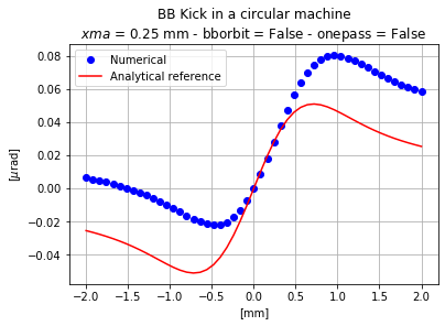
The results are shown below, leaving the onepass argument to False.

png png

In this case, the dipolar effect of the beam-beam element is not taken into consideration and therefore the zero amplitude particle does not receive any kick. On the other hand, particles with $x > 0$ receive a higher kick while the kick given to the particles with negative horizontal position is reduced.

One can now wonder what if the bborbit flag is set to True. We expect that the particle receiving zero kick is the one located ot $x=xma$ . By running:

xma=0.00025
madx.input(
f'''
option,echo=false,warn=false,info=false;
myBB : beambeam, charge=1, sigx={sigma_x}, sigy={sigma_y}, xma={xma}, yma={yma}, bbshape=1, bbdir=-1;

lhc: sequence, l={positionBB};
myBB1: myBB, at={positionBB};
endsequence;

beam, particle=proton, energy={totalEnergy},npart={npart};

use, sequence=lhc;

option, bborbit=true;
twiss,betx={betax_IP},bety={betay_IP};
''');

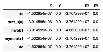
One obtains the following results:

png png

Obvisouly, those results do not match our exepectations. The particle receiving no kick is still the one located at $x = 0$ , and the other particles seem to receive more or less kick depending on their positions.

As seen in the TWISS table, the trajectory of the particle is not modified, but one can now observe a momentum kick at the BB element location.

The way to proceed now is to set the onepass argument to True so MAD-X will not try to compute a closed orbit. As mentionned previously, the CO computation algorithm in the case of a line can be very unstable.

The results are now more consistent:

png png

The particle that does not receive any kick is indeed the particle corresponding to the offset of the strong beam, as it should be.

Note: Once the onepass flag is set to True, the bborbit flag becomes irrelevant. Indeed, the tracking is done in the closed orbit reference. If the latter is not computed, no effect can be expected to be visible. On the other hand, the effect of the bborbit remains visible in the twiss table. With bborbit set to True, a kick is visisble at the BB location, while if bborbit is set to False, the obtained TWISS table is:

png

3) BB Element in a period

As we did for the horizontal kicker, we can now install our BB element in circular machine composed of the same transfer line closed with a rotation matrix.

madx.input(
f'''

myBB : beambeam, charge=+1, sigx={sigma_x}, sigy={sigma_y}, xma={xma}, yma={yma}, bbshape=1, bbdir=-1;
myMatrix: MATRIX, L=0, RM11={RM11}, RM12={RM12}, RM21={RM21}, RM22={RM22},
    RM33={RM33}, RM34={RM34}, RM43={RM43}, RM44={RM44};

lhc: sequence, l={positionBB};
myBB1: myBB, at={positionBB};
myMatrix1: myMatrix, at={positionBB};
endsequence;

beam, particle=proton, energy={totalEnergy}, npart={npart};
use, sequence=lhc;

option, bborbit=false;
twiss;
option,echo=false,warn=false,info=false;
''');

In this example, we set the bborbit flag to False, and as expected we obtain the same plot as in the case of the transfer line without dipolar effect of the beam-beam element.

png

In this case, the closed orbit is vanishing as seen in the TWISS table:

png

If one now adds a similar offset as previously, the kick looks obviously different, but the particle that does not receive any kick is still the one at $x=0$ .

png png

One can modify the bborbit to True and obtain the exact same plot for the kick.

png

But a different TWISS table:

png

This indicates that the tracking is done with respect to the closed orbit while the bborbit flags acts on the closed orbit.

IV - Summary Plot and Warnings

The results obtained in this page are summarized in the following plot.

png

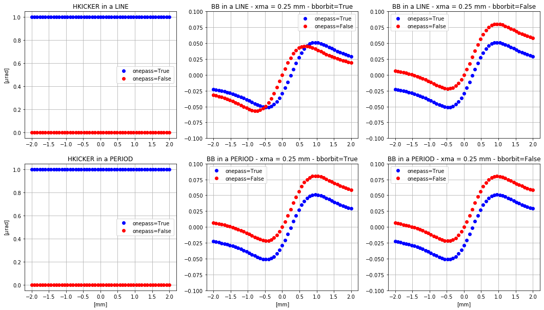
The most important warning that can be taken from this summary is the fact that the dipolar effect processing is done differently depending on its source. For a HKICKER, setting onepass to True allows the user to visualize the dipolar effect in the tracking results while it is not the case for a BB element. More over, even though it is not highlighted in this summary plot, setting the onepass argument to False in the case of a line can be very unstable since MAD-X tries to compute a closed orbit.

Conclusions

In this page, we compared dipolar effects coming from different source and the way MAD-X modules deal with those. In order to understand the process, we compared the installation of a horizontal kicker with a BB element, in both a line and a period.

For the HKICKER, results fit our expectations, and the MAD-X manual. When installing a HKICKER, the kick is visible in the TWISS table and in the TRACK module output if the onepass argument of the TRACK module is set to True. This confirms the MAD-X manual: if onepass is set to True, the particle coordinates are given with respect to the reference orbit while is this argument is set to False, the coordinates are given with respect to the closed orbit.

From the BB installation in a line, a couple of general remarks have been first made. The effect of the BB element is indeed strongly coupled with the definition of the weak beam. On the other hand, it is not possible to include a second strong beam in the sequence to use it in order to define the BB element. As a result, the energy of the opposite beam is assumed to be the same, and its intensity can only modified by changing the charge of the BB element. The energy of the weak beam is important since the BB kick is not normalized to the energy. Finally, the direction of the opposite beam can be changed using the bbrdir. If the BB element always assumes a co-linear beam-beam interaction, changing bbdir to +1 assumes the opposite beam to circulate in the same direction as the weak beam. In that case, since we are dealing with ultra-relativistic beams, the BB kick vanishes.

On the other hand, the dipolar effect of the BB element, visible by setting the bborbit flag to True and adding an offset of the strong beam, is not handled the same was as the HKICKER. If the effect is visible in the TWISS table, it is not true for the TRACK output with onepass set to True. In order to appreciate the effect of those flags on a closed orbit, it was necessary to move from a line to a circular machine or period. This was done by inserting a MATRIX element to close our machine.

We summarize here very important statements that compose our conclusions regarding this study:

If the bborbit flag is set to True, MAD-X will take into consideration the dipolar effect of the beam-beam element on the closed orbit (for a period) or on the trajectory (for a line). This is visible in the TWISS table since the trajectory or the closed orbit are defined with respect to the reference orbit (which exists for both line or period).
In the TRACK module, the onepass argument allows the user to track the particles either with respect to the closed orbit in the case of a period, or with respect to the trajectory in case of a line. Setting this argument properly is therefore important in order to avoid inconsistency in the kick computation. The bborbit flag status will therefore have no effect on the output of the TRACK module.
The dipolar effect of the BB element and the HKICKER are not processed in the same way. For the BB element, setting the onepass argument to True in the case of a line is not enough to see the dipole kick and one should refer also to the TWISS table
The closed orbit computation done when onepass is set to False can be very unstable in the case of a line and is therefore not recommended.

The authors hope that this note will answer some doubts about the BB element implementation and to properly use the different flags/modules to get the desired information. We strongly encourage to share any doubt or problem you might encounter, for further discussion.

References

[1] X. Buffat, "Coherent Beam-Beam Effects", CAS on Intensity Limitations in Particle Beams, Geneva, 2015.