ABP CWG 2020 05 29
NXCALS and pyspark
G. Sterbini with the help and support of the NXCALS team
Introduction
-
We will present few examples on how to use pyspark methods to access NXCALS.
-
pyspark is a ready-to-use package supported by the Apache/SPARK community.
-
pyspark opens the possibility to make big data analysis and could be complementary to pytimber.
Our aim here is to collect examples specific of our community and share them to optimize (and merge in future?) the different approaches.
We are using the SWAN/NXCALS environment but we also tested the pyspark bundle and pure python approach (refer to NXCALS web page).
We are NOT SPARK experts but these examples (of incremental complexity) may bootstrap the discussion and help to build your own use-case.
For our purpose, we privileged the clarity/compactness of code to the completeness of the physics case.
The logic
Given a time window (two ordered timestamps) and a list of variables, one can follow 4 logic steps/sets of dataframes (df): 1. Prepare a set of single spark df's (one per variable). 2. Join this set in a common spark df. 3. Perform transformation on the common spark df. 4. Retrieve a reduced spark df converting it to pandas df.
The emphasis is to do all transformation before step 4, hence make use of the NXCALS cluster.
To keep in mind:
-
Working with the injectors data is in general easier (acquisition done by cyclestamp: synchronous acquisition due to strongly-coupled/fixed-duration-cycles/PPM-telegram).
-
Later we will show the more general case, e.g., LHC: asynchronous acquisition (weakly-coupled/no-fixed-duration-cycles/no-telegram)
An auxiliary package
We put on https://github.com/sterbini/nx2pd (98 sloc) some recurrent functions we are going to use.
import matplotlib
matplotlib.rc('xtick', labelsize=20)
matplotlib.rc('ytick', labelsize=20)
from matplotlib import pyplot as plt
plt.rcParams.update({'font.size': 22})
from nx2pd import nx2pd as nx #install from https://github.com/sterbini/nx2pd
nx.spark=spark
pd=nx.pd
np=nx.np
Example 1a (no transformation)
Q: When and for which cycle a specific PS wire scanner was used?
In this example we are not making transformation (so we are not using the cluster in a smart way).
t1=pd.Timestamp('2018', tz='UTC')
t2=pd.Timestamp('2019', tz='UTC')
list_of_variables=['CPS.LSA:CYCLE','PR.BWS.65.H_ROT:SCAN_NUMBER']
# Step 1: set of single spark df's
pd_df_of_spark_df=nx.importNXCALS(list_of_variables, t1,t2)
# Step 2: inner-joining the pd_df on 'timestamp'
spark_df=nx._join_df_list(pd_df_of_spark_df, on=['timestamp'], how='inner')
# Step 3: going back to pandas df
# Nothing :(
# Step 4: going back to pandas df
pd_df=nx._to_pandas(spark_df, timestampConversion=True, sorted=True)
print(pd_df.head());print(f'A total of {len(pd_df)} records retrieved.')
                                 CPS.LSA:CYCLE  PR.BWS.65.H_ROT:SCAN_NUMBER
2018-03-05 14:43:51.900000+00:00    EAST_IRRAD                        46766
2018-03-05 14:44:35.100000+00:00    EAST_IRRAD                        46767
2018-03-07 08:41:18.300000+00:00    EAST_IRRAD                        46768
2018-03-07 08:41:48.300000+00:00    EAST_IRRAD                        46769
2018-03-10 09:50:08.700000+00:00   MTE_50_CORE                        46770
A total of 15829 records retrieved.
Example 1b (with aggregation)
Q: Same question, when and for which cycle a specific PS wire scanner was used?
(now using aggregation)
t1=pd.Timestamp('2018', tz='UTC')
t2=pd.Timestamp('2019', tz='UTC')
list_of_variables=['CPS.LSA:CYCLE','PR.BWS.65.H_ROT:SCAN_NUMBER']
# Step 1: set of single spark df's
pd_df_of_spark_df=nx.importNXCALS(list_of_variables, t1,t2)
# Step 2: inner-joining the pd_df on 'timestamp'
spark_df=nx._join_df_list(pd_df_of_spark_df, on=['timestamp'], how='inner')
# Step 3: aggregating the data
spark_df=spark_df.groupby('CPS@LSA:CYCLE').agg(nx.func.count("PR@BWS@65@H_ROT:SCAN_NUMBER").alias('count'))
# Step 4: going back to pandas df
pd_df=nx._to_pandas(spark_df,sorted=False).sort_values('count',ascending=False).set_index('CPS.LSA:CYCLE');pd_df.index.name=None;
print(pd_df.head(5));print(f'A total of {len(pd_df)} records retrieved.')
                                   count
MD4263_LHC25#48B_BCMS_PS_TFB_2018   2101
MD4404_BCMS                         1967
MD2586_LHC25#12B_BCMS_PS            1684
LHC25#48B_BCMS_PS                   1064
MD4407_LHC25#12B_BCMS                849
A total of 108 records retrieved.
Example 2a (3 years aggregation)
Q: What is the statistics of the production cycles (first injection current) in the PS during Run2?
You can do that in less than 1 minutes in 2020/05/29 SWAN standard configuration!
t1=pd.Timestamp('2016', tz='UTC'); t2=pd.Timestamp('2019', tz='UTC')
pd_df=nx.importNXCALS(['CPS.TGM:USER','PR.DCAFTINJ_1:INTENSITY'], t1,t2)
df=nx._join_df_list(pd_df, on=['timestamp'], how='inner')
df=df.dropna()\
    .groupby('CPS@TGM:USER').agg(nx.func.count("PR@DCAFTINJ_1:INTENSITY").alias('count'),\
                                    nx.func.sum("PR@DCAFTINJ_1:INTENSITY"),\
                                    nx.func.mean("PR@DCAFTINJ_1:INTENSITY"))
aux=nx._to_pandas(df)
aux=aux.sort_values('CPS.TGM:USER').set_index('CPS.TGM:USER').sort_values('sum(PR.DCAFTINJ_1:INTENSITY)', ascending=False)
aux.index.name=None;print(aux.head());print(f'Total number of cycles: {aux["count"].sum()}')
           count  sum(PR.DCAFTINJ_1:INTENSITY)  avg(PR.DCAFTINJ_1:INTENSITY)
TOF      7785564                  5.312979e+09                    682.414171
SFTPRO1  2972325                  3.270464e+09                   1100.304861
SFTPRO2  2242740                  1.862863e+09                    830.619392
EAST1    3814038                  1.044577e+09                    273.876976
EAST2    3677046                  1.008520e+09                    274.274491
Total number of cycles: 54628119
Example 2b (1 minute aggregation)
CAVEAT: clearly it is faster but, as expected, there are overheads.
t1=pd.Timestamp('2018-10-01', tz='UTC'); t2=pd.Timestamp('2018-10-01 00:01', tz='UTC')
pd_df=nx.importNXCALS(['CPS.TGM:USER','PR.DCAFTINJ_1:INTENSITY'], t1,t2)
df=nx._join_df_list(pd_df, on=['timestamp'], how='inner')
df=df.dropna()\
    .groupby('CPS@TGM:USER').agg(nx.func.count("PR@DCAFTINJ_1:INTENSITY").alias('count'),\
                                    nx.func.sum("PR@DCAFTINJ_1:INTENSITY").alias('sum'),\
                                    nx.func.mean("PR@DCAFTINJ_1:INTENSITY").alias('mean'),\
                                    nx.func.stddev("PR@DCAFTINJ_1:INTENSITY").alias('std'))
aux=nx._to_pandas(df)
aux=aux.sort_values('CPS.TGM:USER').set_index('CPS.TGM:USER').sort_values('sum', ascending=False)
aux.index.name=None;print(aux.head());print(f'Total number of cycles: {aux["count"].sum()}')
         count           sum         mean         std
SFTPRO1      8  11461.413086  1432.676636   18.081495
TOF          8   6481.819397   810.227425    9.617653
EAST1        7   2806.542114   400.934588    2.437349
EAST2        4    880.980518   220.245130  208.533554
MD6          2    156.822815    78.411407    5.531555
Total number of cycles: 35
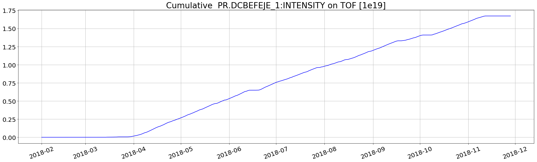
Example 3 (daily cumulative aggregation)
Q: plot the integrated daily extracted current on PS TOF cycle for the 2018
We make explicit operation on the column 'timestamp' before aggregation and we use filtering.
t1=pd.Timestamp('2018', tz='UTC')
t2=pd.Timestamp('2019', tz='UTC')
pd_df=nx.importNXCALS(['CPS.TGM:USER','PR.DCBEFEJE_1:INTENSITY'], t1,t2)
df=nx._join_df_list(pd_df, on=['timestamp'], how='inner')
df=df.filter(nx.col('CPS@TGM:USER')=='TOF')
df=df.withColumn('new_timestamp',nx.col('timestamp')/1.0e9)
df = df.withColumn('new_timestamp',nx.func.from_unixtime("new_timestamp", "yyyy-MM-dd HH:mm:ss"))
df_agg = df.groupBy(nx.func.to_date('new_timestamp').alias('Day')).agg(nx.func.sum('PR@DCBEFEJE_1:INTENSITY').alias('value'))
# to pandas
aux=nx._to_pandas(df_agg)
# minimal operation in pandas after aggregation
aux=aux.sort_values('Day').set_index('Day');aux.index.name=None
plt.figure(figsize=(30,8))
plt.plot(aux['value'].cumsum()/1e9,'-b')
plt.title('Cumulative  PR.DCBEFEJE_1:INTENSITY on TOF [1e19]')
plt.xticks(rotation=20);
plt.grid()
Example 4 (cyclestamps arithmetic)
Q: What is the efficiency of transmission between PSB and PB for TOF?
Cyclestamps arithmetic can be used to "follow" a beam in the injector chain.
HINT: "consecutive" cyclestamps from PS and PSB are 635 ms apart.
t1=pd.Timestamp('2018-10-01 00:00', tz='UTC')
t2=pd.Timestamp('2018-10-01 00:05', tz='UTC')
pd_df=nx.importNXCALS(['CPS.TGM:USER','PR.DCAFTINJ_1:INTENSITY'], t1,t2)
df=nx._join_df_list(pd_df, on=['timestamp'], how='inner')
df_ps=df.filter(nx.col('CPS@TGM:USER')=='TOF').filter(nx.col('PR@DCAFTINJ_1:INTENSITY')>500.)

pd_df=nx.importNXCALS(['PSB.TGM:USER','BR2.BCT.ACC:INTENSITY'], t1,t2)
df=nx._join_df_list(pd_df, on=['timestamp'], how='inner')
df_psb=df.withColumn('timestamp',nx.col('timestamp')+635000000) # cyclestamps arithmetic

out=nx._join_df_list([df_ps,df_psb],how='inner')
out=out.withColumn('efficiency',nx.col('PR@DCAFTINJ_1:INTENSITY')/nx.col('BR2@BCT@ACC:INTENSITY'))
print(nx._to_pandas(out, timestampConversion=False, sorted=True)[['CPS.TGM:USER','PSB.TGM:USER','efficiency']].head())
                    CPS.TGM:USER PSB.TGM:USER  efficiency
1538352006700000000          TOF          TOF    0.980367
1538352010300000000          TOF          TOF    0.977946
1538352013900000000          TOF          TOF    0.980870
1538352028300000000          TOF          TOF    0.979842
1538352035500000000          TOF          TOF    0.981096
Example 5 (UDF scalars to scalar)
In the previous example we compute the efficiency just dividing columns. In general, for more complex, function we can use a User Defined Function.
# %% UDF scalars to scalar
# This function compute the transmission efficiency between injection and extraction of the PS
def my_efficiency(current_inj,current_eje):
    if current_inj>0:
        aux=current_eje/current_inj
    else:
        aux=0.    # it is important to force the double for NXCALS
    if aux<0:
        return 0. # it is important to force the double for NXCALS
    else:
        return aux
my_udf = nx.func.udf(my_efficiency, nx.DoubleType())

t1=pd.Timestamp('2018', tz='UTC')
t2=pd.Timestamp('2019', tz='UTC')
pd_df=nx.importNXCALS(['CPS.TGM:USER','PR.DCAFTINJ_1:INTENSITY','PR.DCBEFEJE_1:INTENSITY'], t1,t2)
spark_df=nx._join_df_list(pd_df, on=['timestamp'], how='inner')
spark_df=spark_df.withColumn('transmission efficiency',my_udf(nx.col('PR@DCAFTINJ_1:INTENSITY'),nx.col('PR@DCBEFEJE_1:INTENSITY')))

aux=nx._to_pandas(spark_df.dropna()\
    .filter(nx.col("PR@DCAFTINJ_1:INTENSITY")>2)\
    .groupby('CPS@TGM:USER').agg(nx.func.count("transmission efficiency").alias('count'),\
                                    nx.func.mean("transmission efficiency").alias('Out/In PS efficiency')))
aux=aux.sort_values('CPS.TGM:USER').set_index('CPS.TGM:USER');aux.index.name=None;print(aux.head())
         count  Out/In PS efficiency
AD      112549              0.988969
EAST1  1166882              0.990395
EAST2  1145499              0.992629
ION1     53903              0.952219
ION2     29311              0.793609
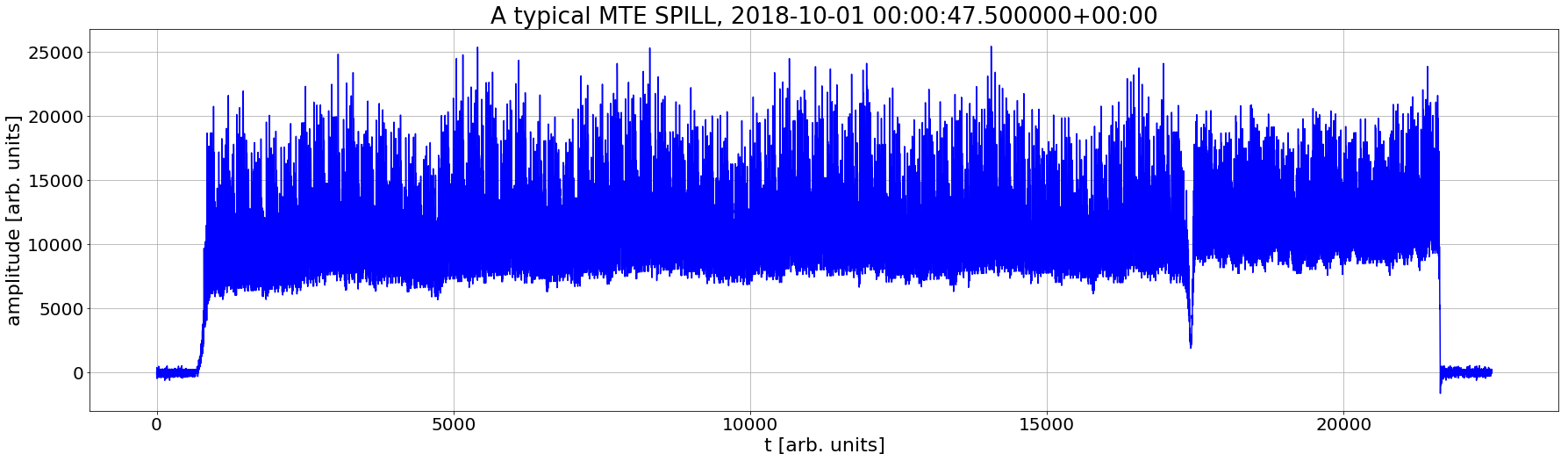
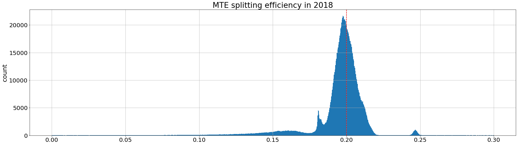
Example 6 (UDF vector to scalar)
Q: Histogram of the multi-Turn Extraction efficiency in 2018
A natural extensions is to compress vector information to scalars.
t1=pd.Timestamp('2018-10-01', tz='UTC')
t2=pd.Timestamp('2018-10-01 00:01', tz='UTC')
df=nx.importNXCALS(['CPS.TGM:USER','PR.SCOPE48.CH01:MTE_SPILL'], t1,t2)
spark_df=nx._join_df_list(df, on=['timestamp'], how='inner')
spark_df=spark_df.filter(nx.col('CPS@TGM:USER')=='SFTPRO1')
plt.figure(figsize=(30,8))
my_row=spark_df.take(2)[0]
plt.plot(my_row['PR@SCOPE48@CH01:MTE_SPILL'],'b')
plt.title(f'A typical MTE SPILL, {pd.Timestamp(my_row["timestamp"]).tz_localize("UTC")}') # it is a heavy signal (>20k samples)
plt.xlabel('t [arb. units]');plt.ylabel('amplitude [arb. units]');plt.grid(True)
t1=pd.Timestamp('2018-10-01', tz='UTC')
t2=pd.Timestamp('2018-10-01 00:01', tz='UTC')
df=nx.importNXCALS(['CPS.TGM:USER','CPS.LSA:CYCLE','PR.SCOPE48.CH01:MTE_SPILL','PR.SCOPE48.CH01:MTE_EFFICIENCY'], t1,t2)
df=nx._join_df_list(df, on=['timestamp'], how='inner')
df=df.filter(nx.col('CPS@TGM:USER')=='SFTPRO1')
df.limit(5).show()
+-------------------+------------+-------------+-------------------------+------------------------------+
|          timestamp|CPS@TGM:USER|CPS@LSA:CYCLE|PR@SCOPE48@CH01:MTE_SPILL|PR@SCOPE48@CH01:MTE_EFFICIENCY|
+-------------------+------------+-------------+-------------------------+------------------------------+
|1538352047500000000|     SFTPRO1|    MTE_2018_|     [-124.17984259390...|                  0.1969342292|
|1538352046300000000|     SFTPRO1|    MTE_2018_|     [160.132474568082...|                  0.1974465434|
|1538352003100000000|     SFTPRO1|    MTE_2018_|     [-348.93102797674...|                  0.1991091949|
|1538352031900000000|     SFTPRO1|    MTE_2018_|     [-127.18853975281...|                  0.1994075732|
|1538352004300000000|     SFTPRO1|    MTE_2018_|     [241.22672082312,...|                  0.1988264771|
+-------------------+------------+-------------+-------------------------+------------------------------+
def MTE_efficiency(myNewSpill):
    b1_idx=2066-1500
    b2_idx=6267-1500
    b3_idx=10468-1500
    b4_idx=14669-1500
    b5_idx=18871-1500
    b6_idx=23072-1500
    is1=np.mean(myNewSpill[b1_idx:b2_idx])
    is2=np.mean(myNewSpill[b2_idx:b3_idx])
    is3=np.mean(myNewSpill[b3_idx:b4_idx])
    is4=np.mean(myNewSpill[b4_idx:b5_idx])
    core=np.mean(myNewSpill[b5_idx:b6_idx])
    mySum=(is1+is2+is3+is4+core);
    MTE_efficiency=np.mean([is1,is2,is3,is4])/mySum;
    return np.float(MTE_efficiency)
my_udf = nx.func.udf(MTE_efficiency, nx.DoubleType())

new_df=df.withColumn('recomputed',my_udf(nx.col('PR@SCOPE48@CH01:MTE_SPILL')))
new_df=new_df.select(['timestamp','PR@SCOPE48@CH01:MTE_EFFICIENCY','recomputed'])
print(nx._to_pandas(new_df, timestampConversion=True, sorted=True).head())
                                  PR.SCOPE48.CH01:MTE_EFFICIENCY  recomputed
2018-10-01 00:00:03.100000+00:00                        0.199109    0.199109
2018-10-01 00:00:04.300000+00:00                        0.198826    0.198826
2018-10-01 00:00:17.500000+00:00                        0.198757    0.198757
2018-10-01 00:00:18.700000+00:00                        0.201958    0.201958
2018-10-01 00:00:31.900000+00:00                        0.199408    0.199408
# about 5 minutes computation
t1=pd.Timestamp('2018', tz='UTC')
t2=pd.Timestamp('2019', tz='UTC')
df=nx.importNXCALS(['CPS.TGM:USER','PR.SCOPE48.CH01:MTE_SPILL','PR.SCOPE48.CH01:MTE_EFFICIENCY'], t1,t2)
df=nx._join_df_list(df, on=['timestamp'], how='inner')
df=df.filter(nx.col('CPS@TGM:USER')=='SFTPRO1')
new_df=df.withColumn('recomputed_MTE_efficiency',my_udf(nx.col('PR@SCOPE48@CH01:MTE_SPILL')))
new_df=new_df.select(['recomputed_MTE_efficiency'])
aux=nx._to_pandas(new_df)
plt.figure(figsize=(30,8))
aux=aux[(aux['recomputed_MTE_efficiency']>0) & (aux['recomputed_MTE_efficiency']<0.3)]
plt.hist(aux['recomputed_MTE_efficiency'].values,1000);
my_ylimit=plt.ylim()
plt.plot([.2,.2],my_ylimit,'--r')
plt.ylim(my_ylimit)
plt.grid()
plt.title('MTE splitting efficiency in 2018')
plt.ylabel('count')
Text(0,0.5,'count')
Example 7 (subsampling and align scalars)
We are going to put all together in our LHC case.
def subSampling(variable,t1,t2,freq='300s'):
    aux=np.array(pd.date_range(t1, t2,freq=freq).astype(np.int64))
    spark_variable=nx._replace_specials(variable)
    pd_df=nx.importNXCALS([variable], t1,t2)
    def set_window(timestamp):
        try:
            return np.int(np.where(aux>timestamp)[0][0])
        except:
            return np.int(0)
    def set_window_time(window):
        try:
            return np.int((aux[window-1]+aux[window])/2)
        except:
            return np.int(0)
    udf_set_window = nx.func.udf(set_window, nx.LongType())
    udf_set_window_time = nx.func.udf(set_window_time, nx.LongType())
    spark_df=nx._join_df_list(pd_df, on=['timestamp'], how='inner')
    spark_df=spark_df.withColumn('window',udf_set_window(nx.col('timestamp')))
    spark_df=spark_df.withColumn('timeWindow',udf_set_window_time(nx.col('window')))
    return spark_df.groupby('window').agg(nx.func.mean(spark_variable).alias(spark_variable),\
        nx.func.count(spark_variable).alias('count_'+spark_variable),\
        nx.func.mean(spark_variable).alias('mean_'+spark_variable),\
        nx.func.stddev(spark_variable).alias('stddev_'+spark_variable),\
        nx.func.min(spark_variable).alias('min_'+spark_variable),\
        nx.func.max(spark_variable).alias('max_'+spark_variable),\
        nx.func.min("timeWindow").alias("timestamp")).drop('window')
t1=pd.Timestamp('2018-10-01', tz='UTC')
t2=pd.Timestamp('2018-10-02', tz='UTC')
my_variable_list=['ALICE:LUMI_TOT_INST','ATLAS:LUMI_TOT_INST','CMS:LUMI_TOT_INST','LHCB:LUMI_TOT_INST']\
    +['LHC.BCTFR.A6R4.B1:BEAM_INTENSITY','LHC.BCTFR.A6R4.B2:BEAM_INTENSITY']\
    +['LHC.BLM.LIFETIME:B1_BEAM_LIFETIME','LHC.BLM.LIFETIME:B2_BEAM_LIFETIME']+['RPMBB.RR17.ROD.A12B1:I_MEAS']
my_spark_variable_list=nx._replace_specials(my_variable_list)
my_list=[subSampling(i,t1,t2) for i in my_variable_list ]
spark_df=nx._join_df_list(my_list, how='outer')
aux=nx._to_pandas(spark_df.select(*my_spark_variable_list,'timestamp'), sorted=True, timestampConversion=True);print(aux[['ALICE:LUMI_TOT_INST','RPMBB.RR17.ROD.A12B1:I_MEAS']].head())
                           ALICE:LUMI_TOT_INST  RPMBB.RR17.ROD.A12B1:I_MEAS
2018-10-01 00:02:30+00:00             3.530905                      -338.99
2018-10-01 00:07:30+00:00             3.541737                      -338.99
2018-10-01 00:12:30+00:00             3.571198                      -338.99
2018-10-01 00:17:30+00:00             3.514797                      -338.99
2018-10-01 00:22:30+00:00             3.455339                      -338.99
Example 8 (putting together, subsampling and align vectors)
To cope with bunch-by-bunch analysis we need to subsample vactors.
def subSamplingVector(variable, t1, t2, my_DatetimeIndex):
    aux=np.array(my_DatetimeIndex.astype(np.int64))
    spark_variable=nx._replace_specials(variable)
    pd_df=nx.importNXCALS([variable], t1,t2)
    def set_window(timestamp):
        try:
            return np.int(np.where(aux>timestamp)[0][0])
        except:
            return np.int(0)
    def set_window_time(window):
        try:
            return np.int((aux[window-1]+aux[window])/2)
            #return np.int(aux[window-1])
        except:
            return np.int(0)
    def compute_mean(x):
        try:
            aux=0
            for i in len(x):
                aux=a+x[i]
            return aux/len(x)
        except:
            return x[0]
    udf_set_window = nx.func.udf(set_window, nx.LongType())
    udf_set_window_time = nx.func.udf(set_window_time, nx.LongType())
    udf_compute_mean = nx.func.udf(compute_mean, nx.ArrayType(nx.DoubleType()))
    spark_df=nx._join_df_list(pd_df, on=['timestamp'], how='inner')
    spark_df=spark_df.withColumn('window',udf_set_window(nx.col('timestamp')))
    spark_df=spark_df.withColumn('timeWindow',udf_set_window_time(nx.col('window')))
    return spark_df.groupby('window').agg(udf_compute_mean(nx.func.collect_list(spark_variable)).alias(spark_variable),\
                                          nx.func.min("timeWindow").alias("timestamp")).drop('window')
And combining the different functions...
t1=pd.Timestamp('2018-10-01', tz='UTC')
t2=pd.Timestamp('2018-10-02', tz='UTC')
my_DatetimeIndex=pd.date_range(t1, t2, freq='300s')
my_variable_list=['LHC.BCTFR.A6R4.B1:BUNCH_INTENSITY','LHC.BCTFR.A6R4.B2:BUNCH_INTENSITY','ATLAS:BUNCH_LUMI_INST','CMS:BUNCH_LUMI_INST',
                  'LHC.BSRT.5R4.B1:BUNCH_EMITTANCE_H',
                  'LHC.BSRT.5R4.B1:BUNCH_EMITTANCE_V',
                  'LHC.BSRT.5L4.B2:BUNCH_EMITTANCE_H',
                  'LHC.BSRT.5L4.B2:BUNCH_EMITTANCE_V']
my_spark_variable_list=nx._replace_specials(my_variable_list)
my_list1=[subSamplingVector(i,t1,t2,my_DatetimeIndex) for i in my_variable_list]

my_variable_list=['ALICE:LUMI_TOT_INST','ATLAS:LUMI_TOT_INST','CMS:LUMI_TOT_INST','LHCB:LUMI_TOT_INST']\
    +['LHC.BCTFR.A6R4.B1:BEAM_INTENSITY','LHC.BCTFR.A6R4.B2:BEAM_INTENSITY']\
    +['LHC.BLM.LIFETIME:B1_BEAM_LIFETIME','LHC.BLM.LIFETIME:B2_BEAM_LIFETIME']+['RPMBB.RR17.ROD.A12B1:I_MEAS']
my_spark_variable_list=nx._replace_specials(my_variable_list)
my_list2=[subSampling(i,t1,t2) for i in my_variable_list ]

my_list3=nx.importNXCALS(['LHC.RUNCONFIG:IP1-XING-V-MURAD',
 'LHC.RUNCONFIG:IP2-XING-V-MURAD',
 'LHC.RUNCONFIG:IP5-XING-H-MURAD',
 'LHC.RUNCONFIG:IP8-XING-H-MURAD']+['HX:BETASTAR_IP1', 'HX:BETASTAR_IP2', 'HX:BETASTAR_IP5', 'HX:BETASTAR_IP8'], t1,t2)

spark_df=nx._join_df_list(my_list1+my_list2+list(my_list3['pyspark df'].values), how='outer')
aux=nx._to_pandas(spark_df, timestampConversion=True, sorted=True); print(aux[['LHC.BSRT.5R4.B1:BUNCH_EMITTANCE_V','LHC.RUNCONFIG:IP2-XING-V-MURAD','ATLAS:LUMI_TOT_INST']].head())
                                                  LHC.BSRT.5R4.B1:BUNCH_EMITTANCE_V  \
2018-10-01 00:02:30+00:00         [0.0, 0.0, 0.0, 0.0, 0.0, 0.0, 0.0, 0.0, 0.0, ...
2018-10-01 00:07:30+00:00         [0.0, 0.0, 0.0, 0.0, 0.0, 0.0, 0.0, 0.0, 0.0, ...
2018-10-01 00:12:30+00:00         [0.0, 0.0, 0.0, 0.0, 0.0, 0.0, 0.0, 0.0, 0.0, ...
2018-10-01 00:14:20.149000+00:00                                               None
2018-10-01 00:17:30+00:00         [0.0, 0.0, 0.0, 0.0, 0.0, 0.0, 0.0, 0.0, 0.0, ...

                                  LHC.RUNCONFIG:IP2-XING-V-MURAD  \
2018-10-01 00:02:30+00:00                                    NaN
2018-10-01 00:07:30+00:00                                    NaN
2018-10-01 00:12:30+00:00                                    NaN
2018-10-01 00:14:20.149000+00:00                             NaN
2018-10-01 00:17:30+00:00                                    NaN

                                  ATLAS:LUMI_TOT_INST
2018-10-01 00:02:30+00:00                12800.725273
2018-10-01 00:07:30+00:00                12692.731878
2018-10-01 00:12:30+00:00                12588.781626
2018-10-01 00:14:20.149000+00:00                  NaN
2018-10-01 00:17:30+00:00                12518.875661
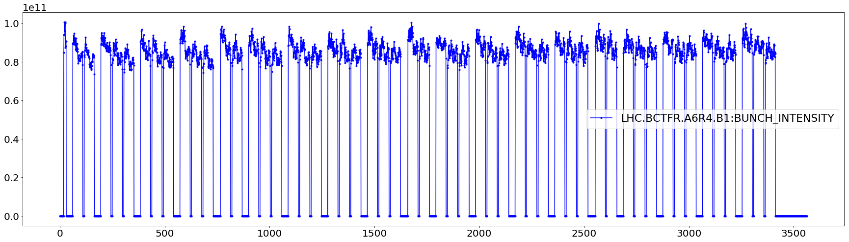
# Few checks
plt.figure(figsize=(30,8))
plt.plot(aux.iloc[0]['LHC.BCTFR.A6R4.B1:BUNCH_INTENSITY'],'.-b', label='LHC.BCTFR.A6R4.B1:BUNCH_INTENSITY')
plt.legend(loc='best')
<matplotlib.legend.Legend at 0x7fa2840c0438>
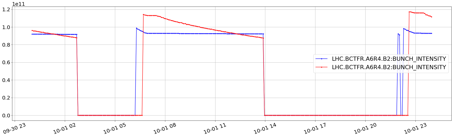
# Few checks
plt.figure(figsize=(30,8))
plt.plot(aux['LHC.BCTFR.A6R4.B2:BUNCH_INTENSITY'].dropna().apply(lambda x:x[6]),'.b-')
plt.plot(aux['LHC.BCTFR.A6R4.B2:BUNCH_INTENSITY'].dropna().apply(lambda x:x[2000]),'.r-')
plt.legend(loc='best')
plt.grid()
plt.xticks(rotation=20);
Example 9 (write/read on HDFS)
Writing and reading to/from HDFS allows us to use SPARK also for the postprocessed data (maintaining the same workflow).
# to write
if 0:
    # very important to repartition to limit the number of files (for a single fill we will repartition to 1 file)
    spark_df.repartition(1).write.mode("overwrite").parquet("fill2.parquet")
You can check the hdfs path by
!hdfs dfs -ls /user/sterbini
Found 6 items
drwx------   - sterbini supergroup          0 2020-05-28 23:20 /user/sterbini/.Trash
drwxr-xr-x   - sterbini supergroup          0 2020-05-29 10:31 /user/sterbini/.sparkStaging
drwxr-xr-x   - sterbini supergroup          0 2020-02-07 14:38 /user/sterbini/bmode
drwxr-xr-x   - sterbini supergroup          0 2020-02-07 14:51 /user/sterbini/bmodes
drwxr-xr-x   - sterbini supergroup          0 2020-05-28 22:40 /user/sterbini/fill1.parquet
drwxr-xr-x   - sterbini supergroup          0 2020-05-28 23:37 /user/sterbini/fill2.parquet
spark_df=spark.read.parquet("fill*.parquet") # Very important
aux=nx._to_pandas(spark_df.select('timestamp','CMS:BUNCH_LUMI_INST'),timestampConversion=True, sorted=True)
print(aux.head())
print(aux.tail())
                                                                CMS:BUNCH_LUMI_INST
2018-10-01 00:02:30+00:00         [-0.002677366, -0.002759958, -0.004399077, -0....
2018-10-01 00:07:30+00:00         [-0.002629694, -0.002912038, -0.005541767, -0....
2018-10-01 00:12:30+00:00         [-0.003120326, -0.002868722, -0.003427472, -0....
2018-10-01 00:14:20.149000+00:00                                               None
2018-10-01 00:17:30+00:00         [-0.001818355, -0.003197438, -0.002672729, -0....
                                                                CMS:BUNCH_LUMI_INST
2018-10-02 23:42:30+00:00         [0.0, 0.0, 0.0, 0.0, 0.0, 0.0, 0.0, 0.0, 0.0, ...
2018-10-02 23:47:30+00:00                                                      None
2018-10-02 23:52:30+00:00                                                      None
2018-10-02 23:53:54.144000+00:00                                               None
2018-10-02 23:57:30+00:00                                                      None
Conclusions
-
We show some examples of pyspark approach we intend to use in our work-flow. We touched only the surface.
-
First impression: we think that NXCALS framework has great potential for the big data analysis.
-
pytimber still fundamental for the typical use (e.g., small data).
Thanks to the NXCALS team for the responsiveness and availability.
Thank you for your attention.